Introduction to Algo Trading for Beginners

[Tradehull_Imran]

Hi @Everyone,

A step-by-step walkthrough of Dhan’s Algo Trading API — from your first live data pull to a fully installed Python trading environment.

---

Overview

This is Part 1 of a five-part series that takes a trader from manual trading to a fully automated, self-built algo. No prior programming background is required — everything is built up gradually, starting with the most basic building block of algo trading: the API.

By the end of the series, you will be able to:

1. Pull live market data and install all required algo files (this part)
2. Learn Python fundamentals for trading
3. Build a momentum scanner using the algo
4. Place orders and deploy the algo on Dhan Cloud
5. Extend the same algo to trade options and deploy it as well

The idea driving the whole series: whatever your strategy — indicator-based, options buying, expiry trading — it can be described to a laptop once in Python, and the laptop will then execute it every day, without manual chart-watching.

Note: No live orders are placed in this part. It covers the API demo and local installation only.

---

1. What Is Algo Trading, Really?

At its core, algo trading comes down to four steps:

• You have a strategy.
• You describe that strategy to your laptop using Python.
• Your laptop talks to your broker (Dhan) using an API.
• Dhan routes your orders to the exchanges (NSE, BSE, MCX) and sends data back the same way.

The API is the communication layer — it’s how a laptop sitting anywhere can “talk” to Dhan’s servers and place orders, pull prices, or manage positions, without a single manual click.

---

2. Live API Demo — What Can the API Actually Do?

Before installing anything, here’s a live walkthrough of the Dhan API from inside the Cursor editor, one call at a time. The examples below use the Dhan-Tradehull wrapper library and the same 50-stock watchlist throughout.

2.1 Live LTP for an Entire Watchlist

A single API call pulls the Last Traded Price (LTP) for the full watchlist — around 50 stocks — in about one second.

ltp_data = tsl.get_ltp_data(names=watchlist)
print(ltp_data)

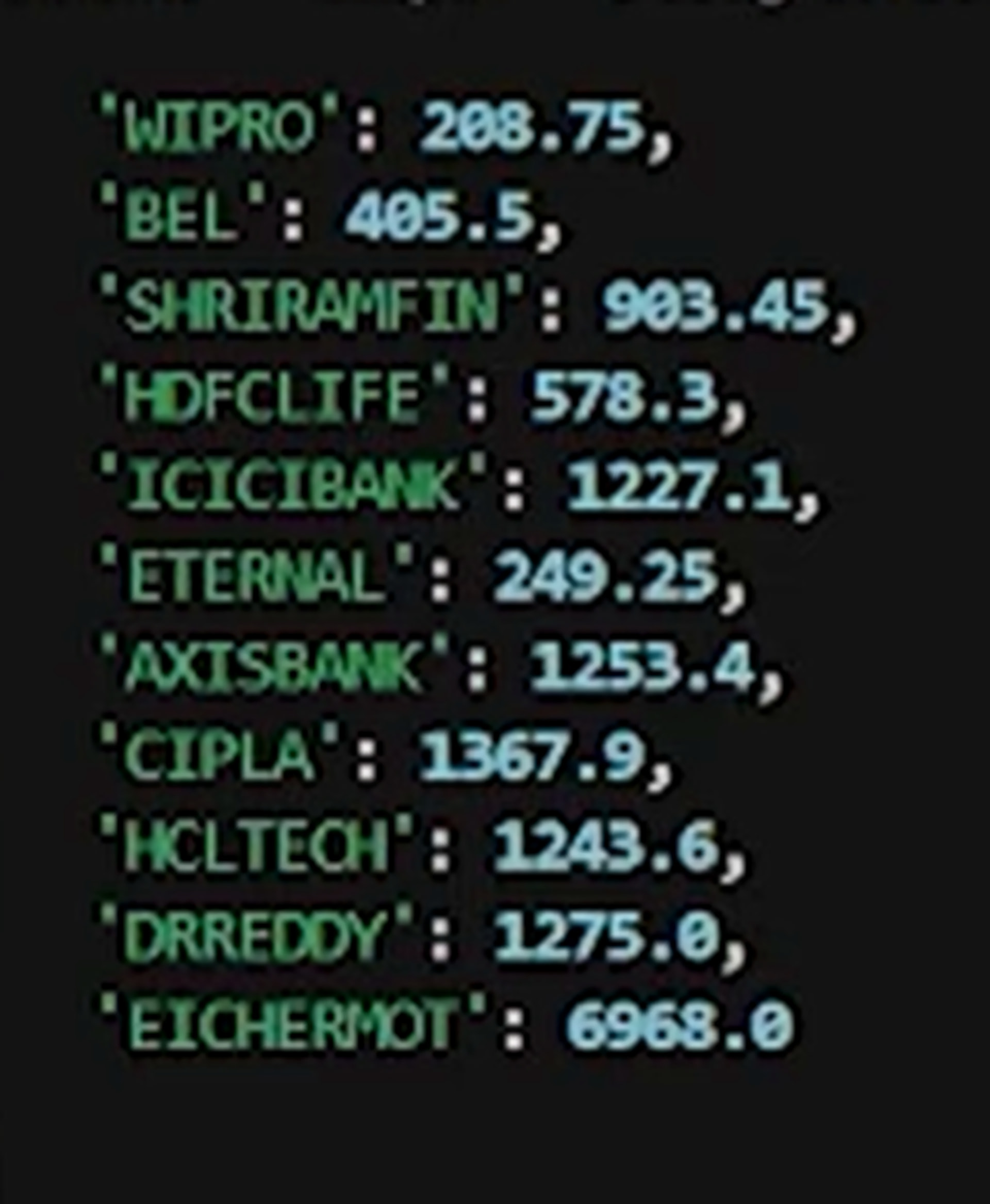
Figure 1: Live LTP pulled for the entire watchlist in a single API call.

2.2 Full Quote Data

Beyond LTP, the same wrapper returns full quote data: 52-week high/low, average price, market depth (buy/sell order book), circuit limits, OHLC, and volume — for every symbol in the watchlist at once.

quote_data = tsl.get_quote_data(names=watchlist)
print(quote_data)

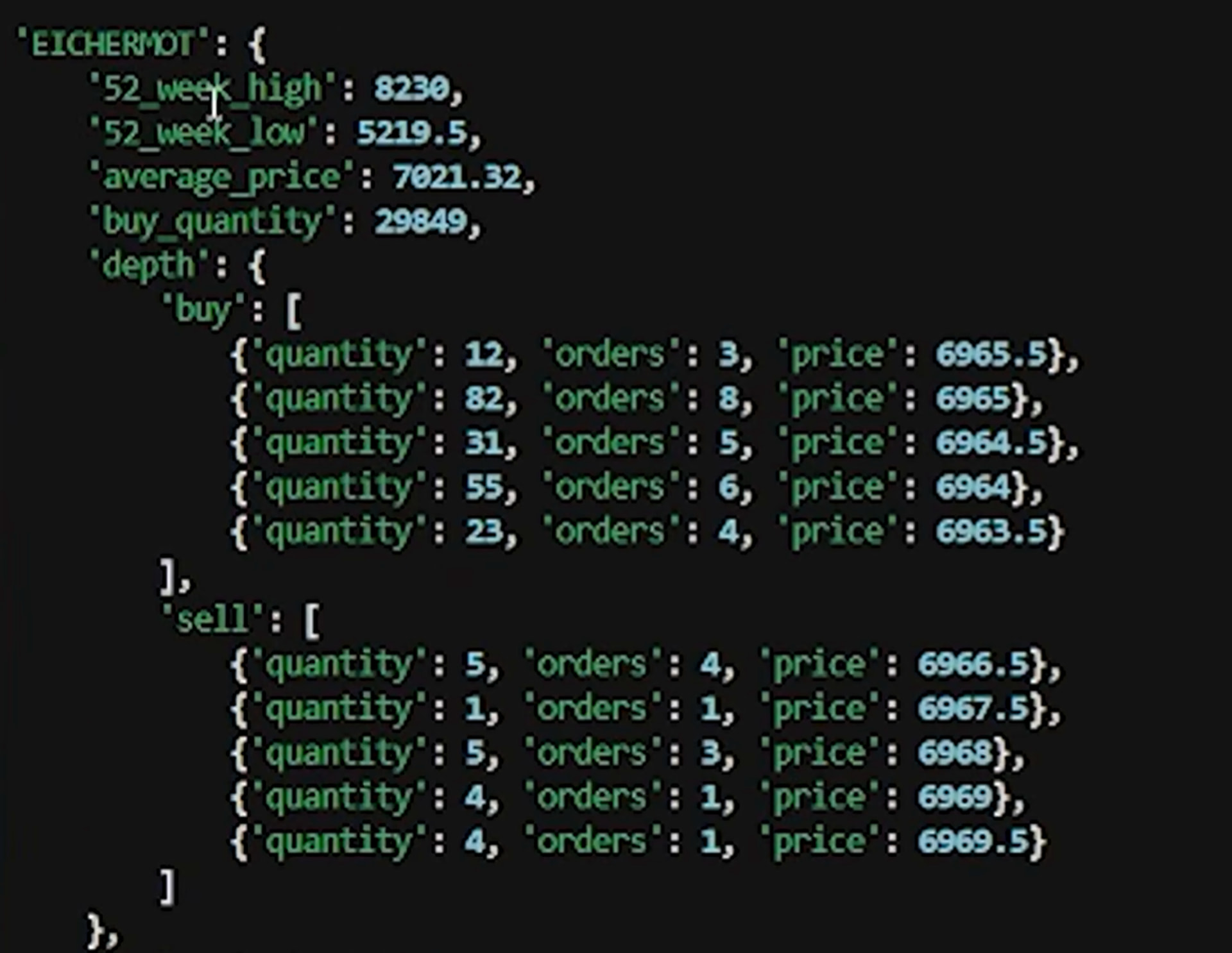
Figure 2: Complete quote data for EICHERMOT — 52-week high/low, average price, and 5-level market depth (buy/sell book).

2.3 Historical & Indicator Data (Nifty, TCS)

The same API fetches historical candle data for any interval — 5-minute Nifty data with an RSI overlay computed via talib, and daily data for individual stocks like TCS, including the previous day’s OHLC (useful for breakout strategies).

nifty_chart = tsl.get_historical_data(tradingsymbol='NIFTY', exchange='INDEX', timeframe="5")
print(nifty_chart)

nifty_chart['rsi'] = talib.RSI(nifty_chart['close'], timeperiod=14)
print(nifty_chart)

tcs_chart = tsl.get_historical_data(tradingsymbol='TCS', exchange='NSE', timeframe="DAY")
print(tcs_chart)

# -1 for the running candle, -2 for the second-last completed candle
tcs_range = tcs_chart.iloc[-1]
print(tcs_range)

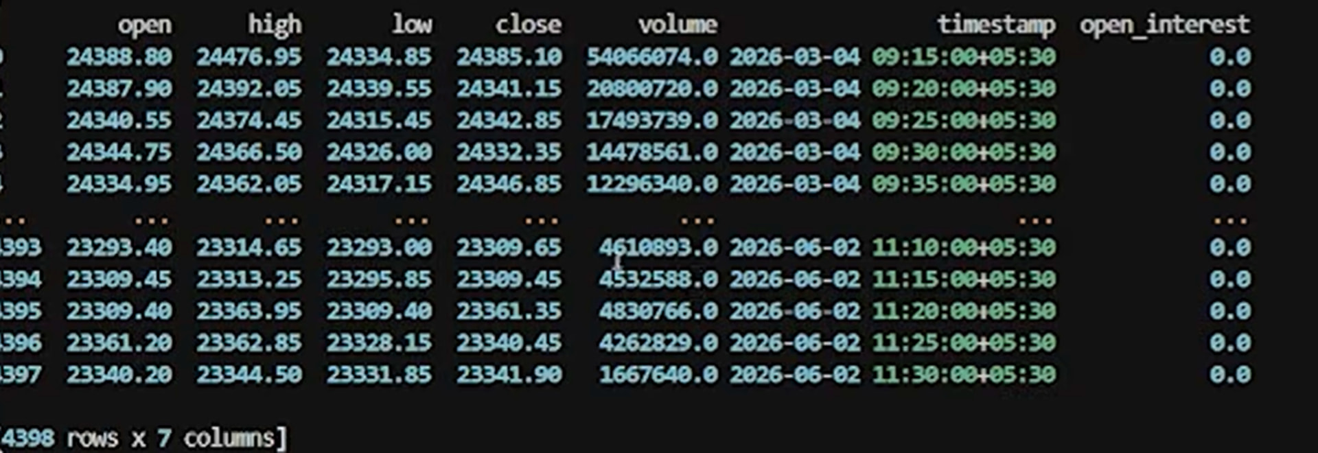
Figure 3: 5-minute Nifty candle data pulled directly through the API — OHLC, volume, and timestamp.

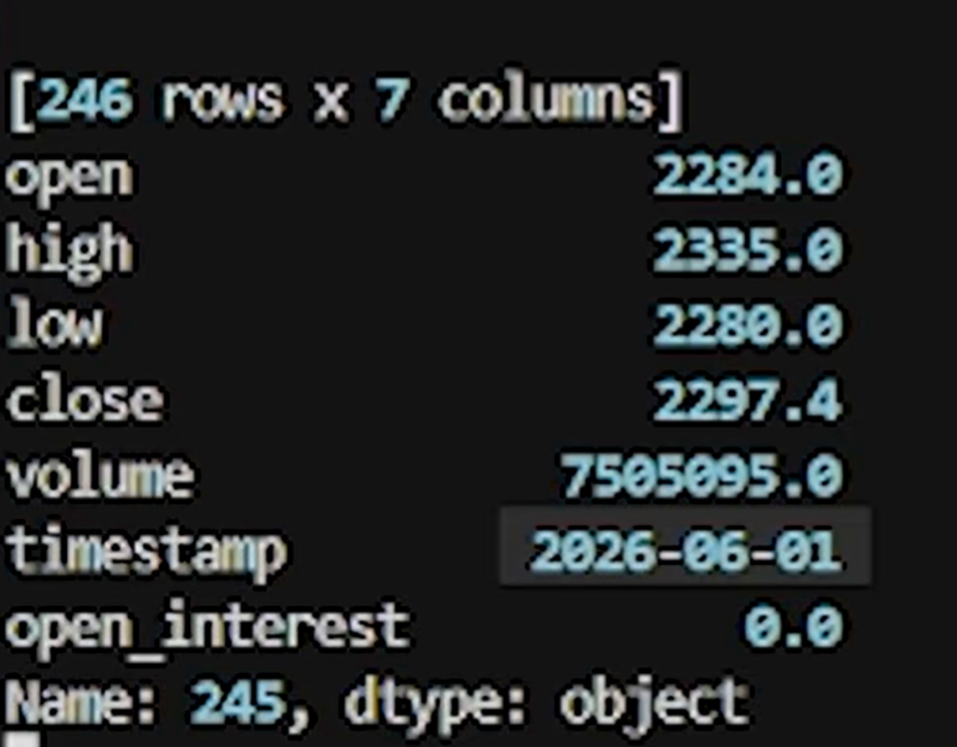
Figure 4: Previous day’s OHLC for TCS, used to plan a breakout-above-prior-high strategy.

2.4 Five Years of Backtesting Data — Reliance

For backtesting, the API can pull years of historical candles in one call — here, 5 years of 5-minute Reliance data (~92,000+ candles), exported straight to CSV.

# Reliance_5_years_backtesting_data.csv must be closed before running
# the to_csv() call below, or the write will fail.
backtesting_data = tsl.get_long_term_historical_data(
    tradingsymbol='RELIANCE',
    exchange='NSE',
    timeframe='5',
    from_date='2021-01-01',
    to_date='2026-05-28'
)
print(backtesting_data)
backtesting_data.to_csv('Reliance 5 years backtesting data.csv')

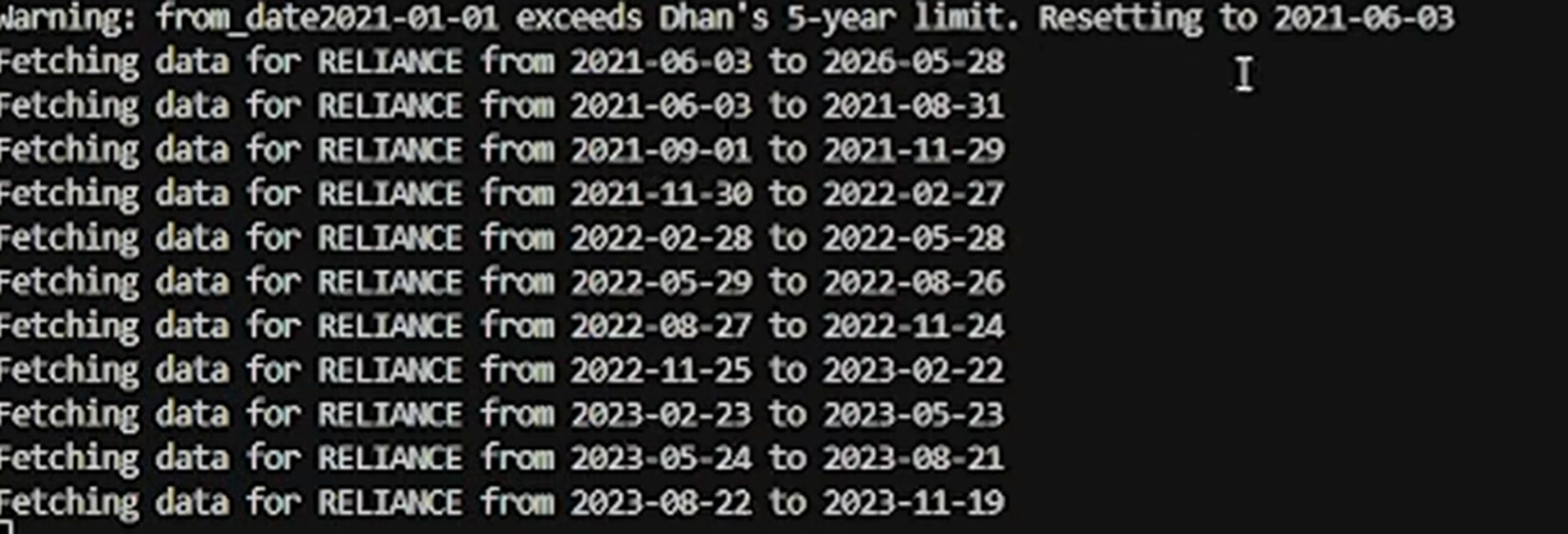
Figure 5: Dhan enforces a 5-year lookback limit — the wrapper automatically chunks the request into ~90-day windows and stitches the result together.

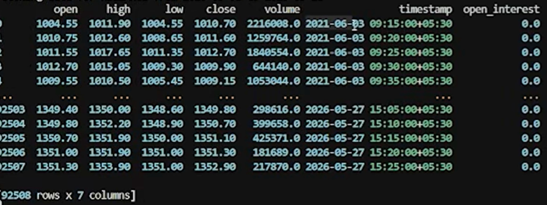
Figure 6: The final stitched dataframe — 92,508 rows spanning June 2021 to May 2026, ready for backtesting.

Opening the exported CSV in a spreadsheet, and rendering it as a candlestick chart, makes the shape of the data easy to check at a glance:

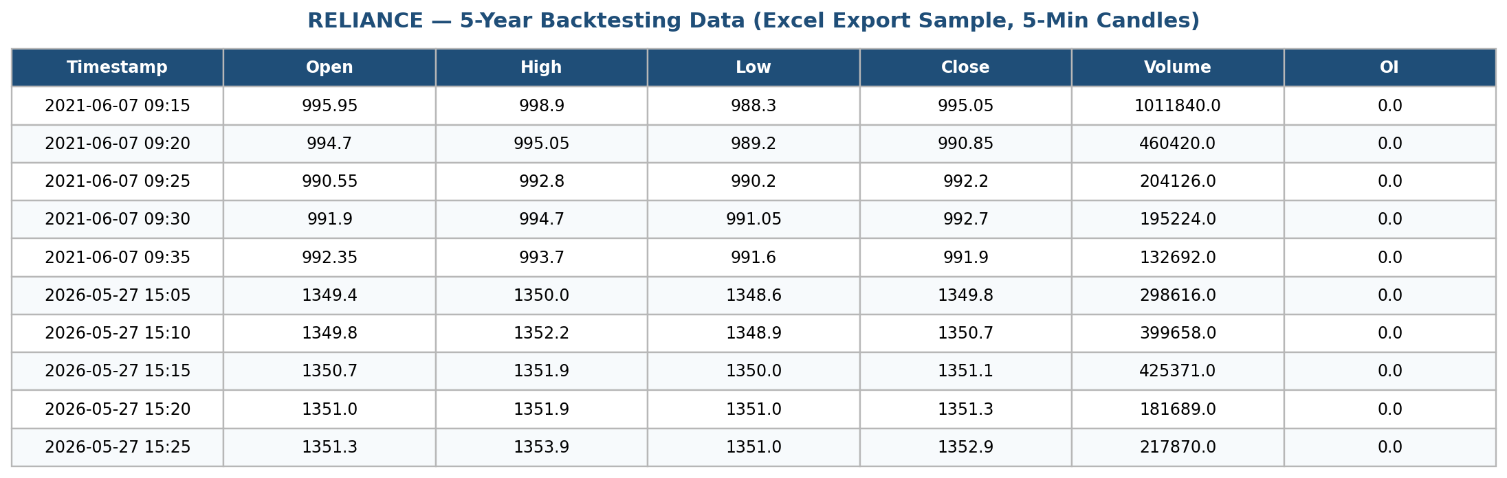
Figure 7: Sample rows (first 5 and last 5) from the exported Reliance_5_years_backtesting_data.csv file.

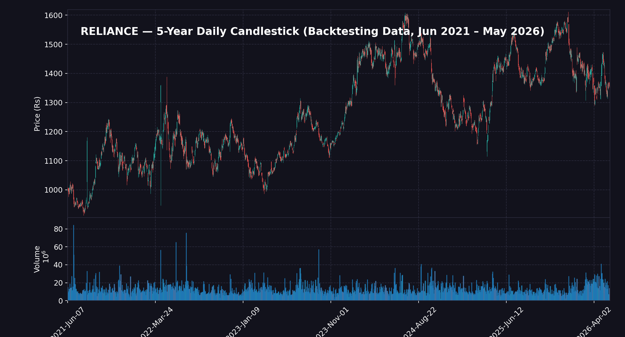
Figure 8: Full 5-year daily candlestick chart built from the exported backtesting CSV — June 2021 to May 2026.

To mirror the RSI + EMA scanner logic used later in this section, here is a recent 5-minute intraday window from the same dataset with EMA(20) and RSI(14) plotted underneath:

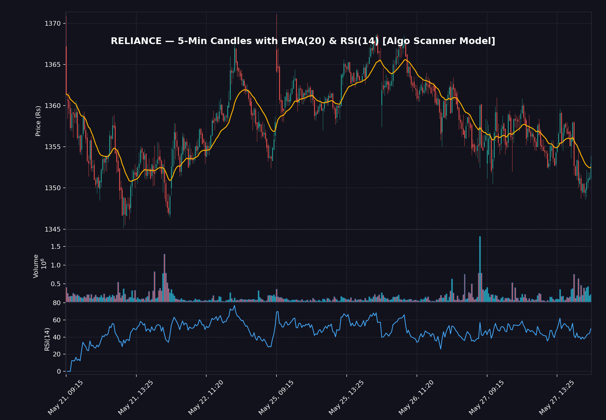
Figure 9: Last ~5 trading sessions of 5-minute Reliance candles with EMA(20) overlay and RSI(14) panel — the same indicator combination used by the RSI/EMA scanner in Section 3.

2.5 Options — ATM / OTM Strike Lookup

The API also resolves At-the-Money (ATM) and Out-of-the-Money (OTM) option strikes directly — you specify the underlying, the expiry, and how many strikes away from ATM you want.

atm_call_name, atm_put_name, atm_strike = tsl.ATM_Strike_Selection(Underlying='NIFTY', Expiry=0)
print(atm_call_name, "\t", atm_put_name, "\t", atm_strike)

otm_call_name, otm_put_name, otm_call_strike, otm_put_strike = tsl.OTM_Strike_Selection(
    Underlying='NIFTY', Expiry=0, OTM_count=5
)
print(
    otm_call_name, "\t", otm_put_name, "\t",
    otm_call_strike, "\t", otm_put_strike
)

Figure 10: ATM call/put and OTM strikes resolved automatically for the current Nifty expiry (23,350 shown as the at-the-money strike).

2.6 Live P&L and Holdings

Live P&L and holdings can be pulled the same way — the foundation for automated risk management such as a max-profit / max-loss auto square-off.

current_pnl = tsl.get_live_pnl()
print(current_pnl)

holdings = tsl.get_holdings()
print(holdings)

Figure 11: Live holdings snapshot — quantity, average cost price, and last traded price per symbol.

Note: Once a max-profit / max-loss threshold is set on Dhan, the platform enables a P&L-based exit for the account — if overall profit or loss crosses that threshold, all open positions are auto-squared-off.

2.7 Complete Option Chain + PCR

The full option chain — every strike, both legs — can be pulled and exported to CSV in one call. Derived metrics like PCR (Put-Call Ratio), or “closest strike to a target LTP / target Delta,” can then be computed directly in Python from that data.

atm, option_chain = tsl.get_option_chain(Underlying="NIFTY", exchange="INDEX", expiry=0, num_strikes=70)
option_chain.to_csv('Option Chain.csv')

pcr = option_chain['PE OI'].sum() / option_chain['CE OI'].sum()
print("PCR : ", pcr)

# Strike with LTP nearest to 30
ltp_based_strike = option_chain.iloc[
    (option_chain['CE LTP'] - 30).abs().argmin()
]
print("strike nearest to 30 : ", ltp_based_strike['Strike Price'])

# Strike with Delta nearest to 0.3
delta_based_strike = option_chain.iloc[
    (option_chain['CE Delta'] - 0.3).abs().argmin()
]
print("Strike below 0.3 Delta: ", delta_based_strike['Strike Price'])

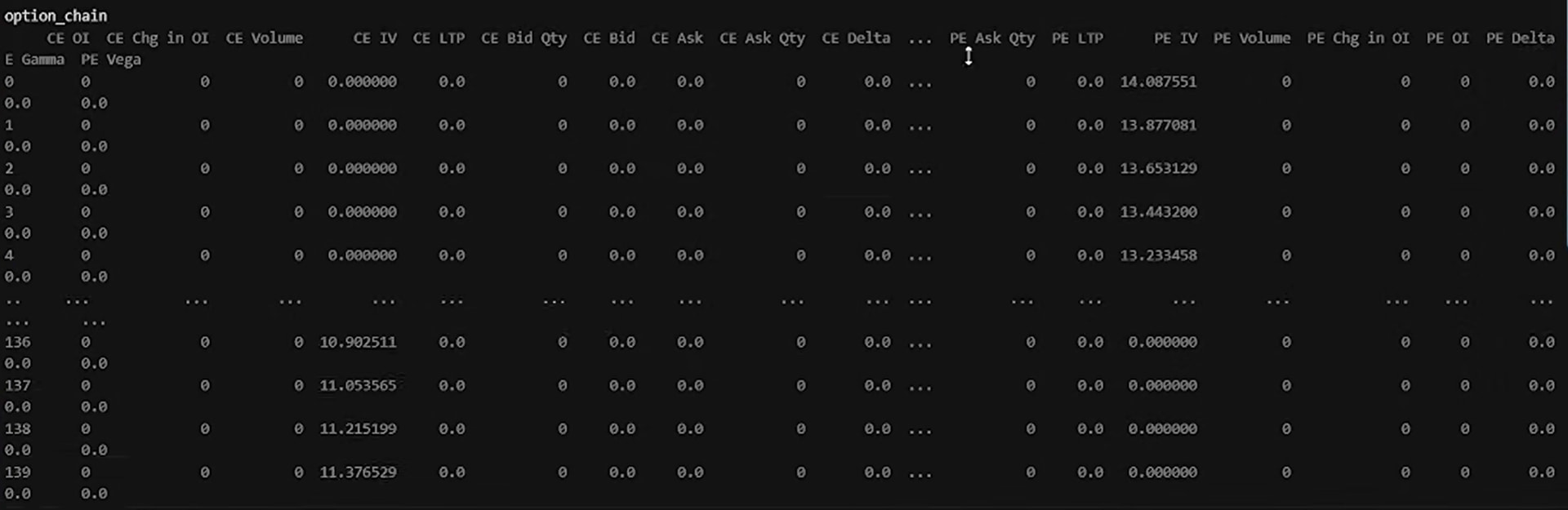
Figure 12: Full Nifty option chain — OI, change in OI, volume, IV, LTP, bid/ask, and Greeks (Delta, Theta, Gamma, Vega) for every strike.

Figure 13: Holdings data alongside a Python-calculated PCR of 0.87 for Nifty — Put OI ÷ Call OI.

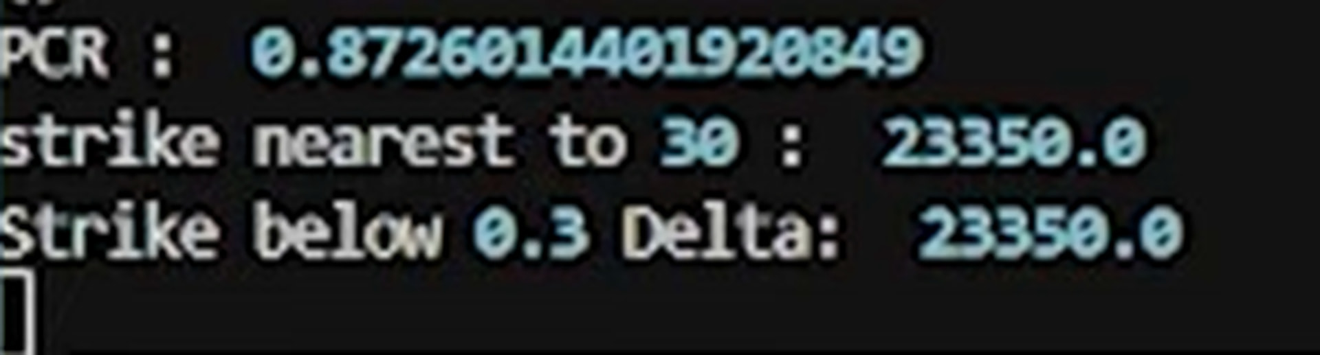
Figure 14: Beyond PCR, the same option chain answers questions like “which strike has an LTP nearest ₹30?” (23,350) or “which strike has a Delta nearest 0.3?” (23,350).

Rendering the exported Option_Chain.csv as charts makes the shape of the chain easy to read at a glance:

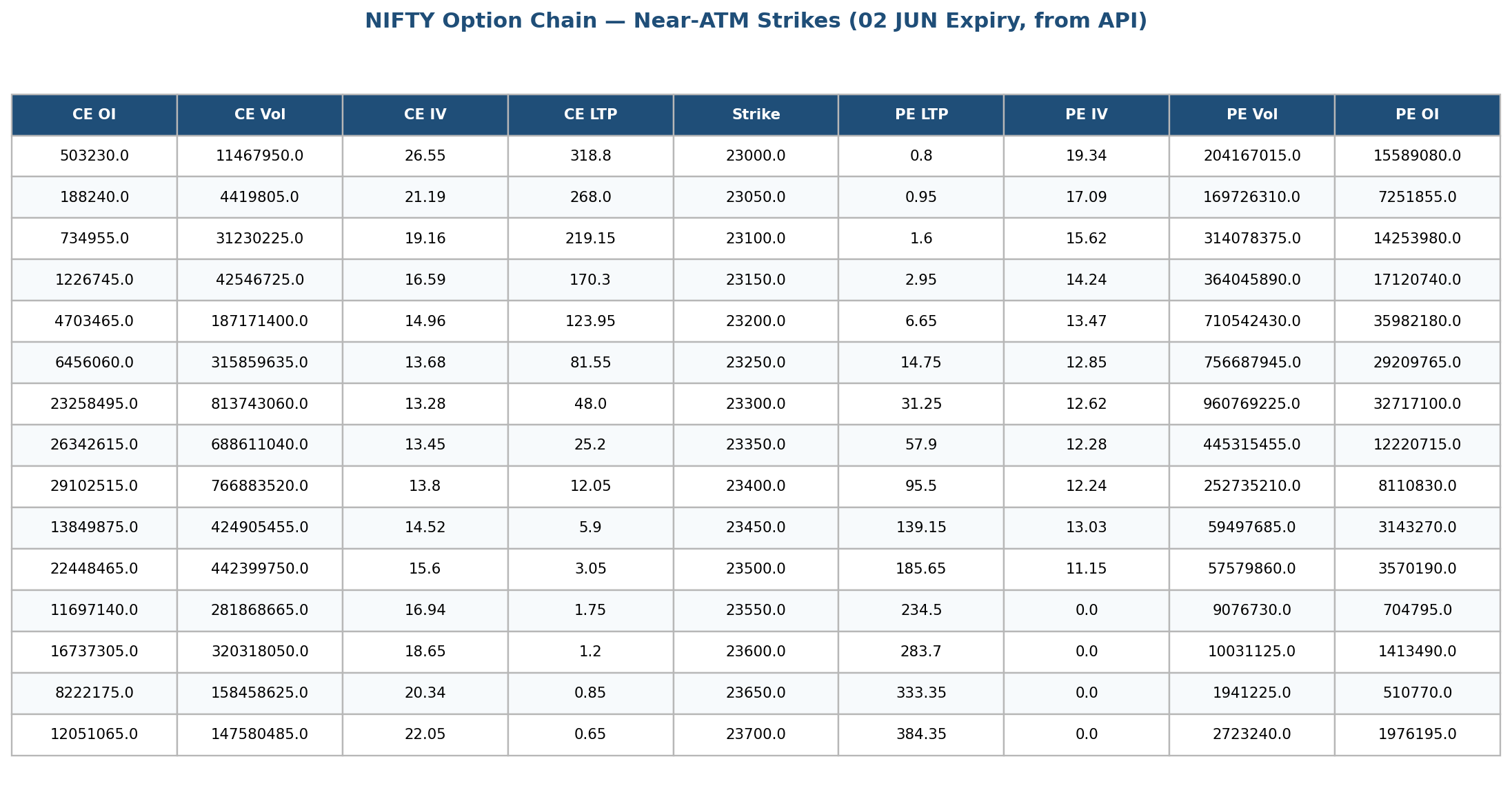
Figure 15: Near-ATM strikes (23,000–23,700) from the exported option chain CSV, formatted as a spreadsheet-style table.

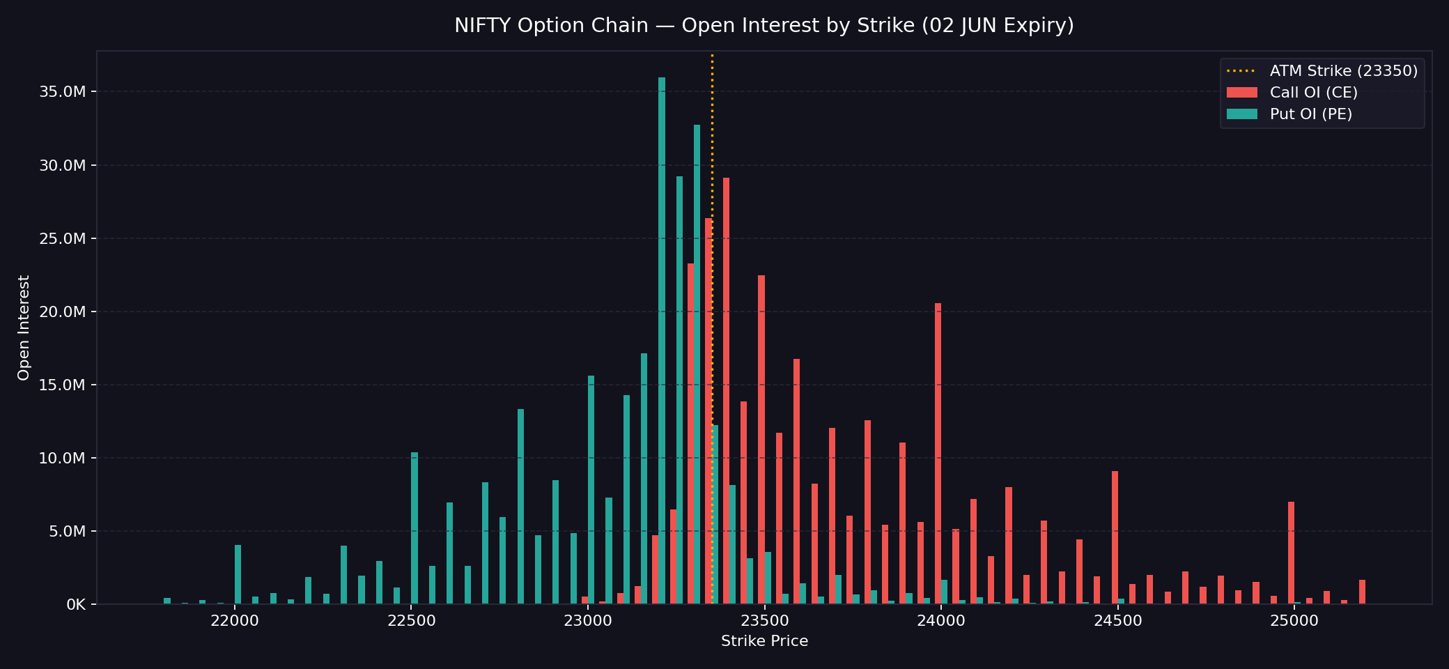
Figure 16: Call OI vs. Put OI by strike, built from the exported option chain data — OI is heavily concentrated at 23,300–23,400, right around the ATM strike.

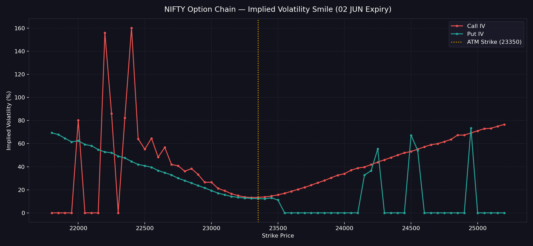
Figure 17: IV smile for the same expiry — implied volatility rises as strikes move away from the ATM zone, characteristic of the volatility skew seen intraday.

2.8 Telegram Alerts

Python can also push Telegram notifications for every algo action — login, entry, position update, trail, or exit — so the algo can be monitored from a phone without watching a terminal all day. This requires creating a personal Telegram bot to get a chat ID and bot token.

tsl.send_telegram_alert(
    message="Order executed: BUY 50 shares of RELIANCE",
    receiver_chat_id="",
    bot_token=""
)

Warning: Never commit a real bot_token or receiver_chat_id to shared code or a public repo — treat them like a password. Generate your own via Telegram’s BotFather and keep them in a local config that isn’t checked into version control.

---

3. Installation — Setting Up Algo Trading on Your Own Laptop

With the API demo covered, the next step is installing everything needed to run this locally. The installation has five steps.

Step 1 — Run the Algo Trader Installer (as Administrator)

Running AlgoTradeInstaller.exe as Administrator downloads and installs Python, the TA-Lib library (for indicators), Pandas TA, XlWings (for Excel control), the Dhan API library, and the TradeHull codebase — all in one pass.

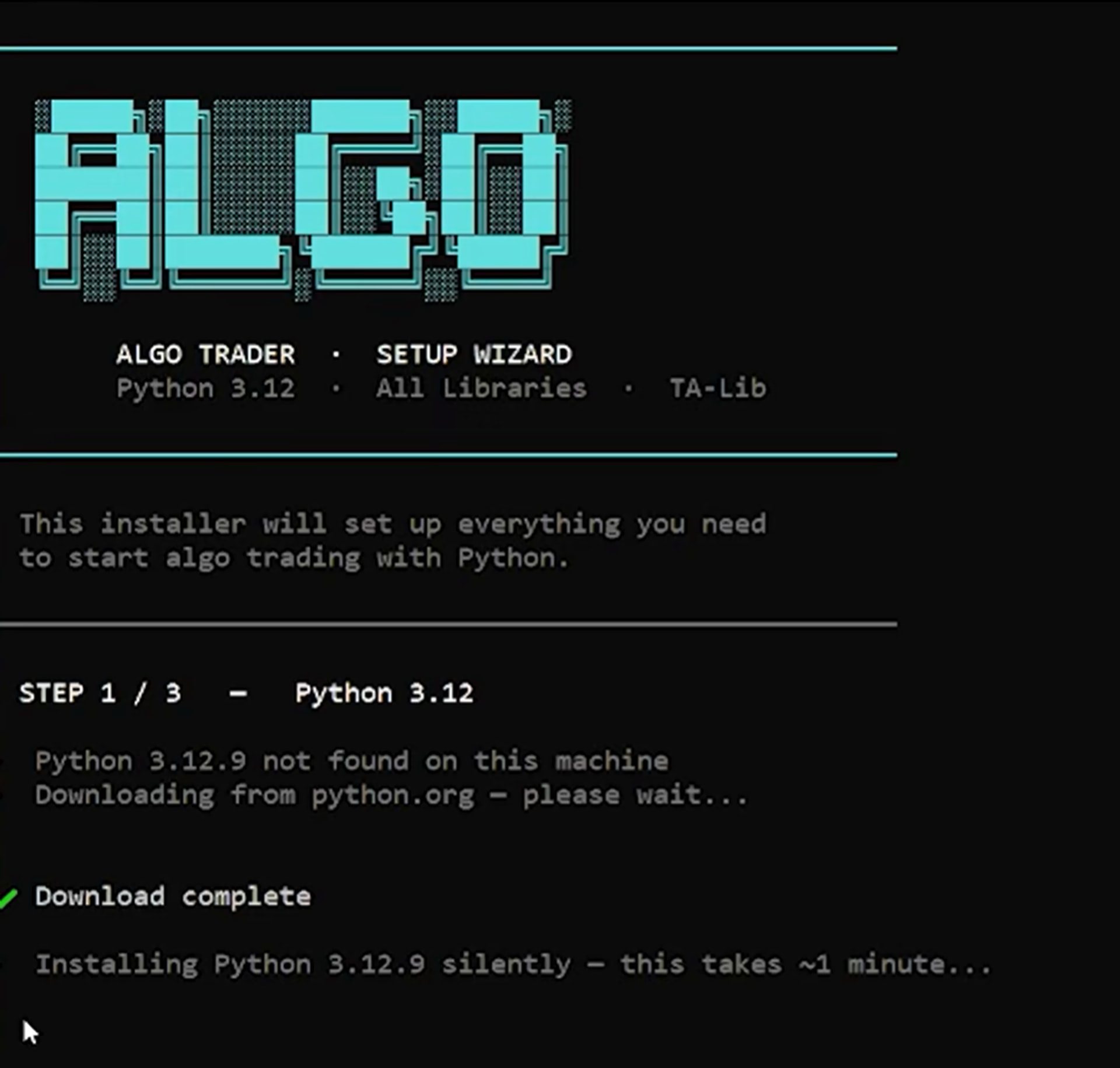
Figure 18: Setup wizard — Python 3.12, all required libraries, and TA-Lib bundled into a single installer.

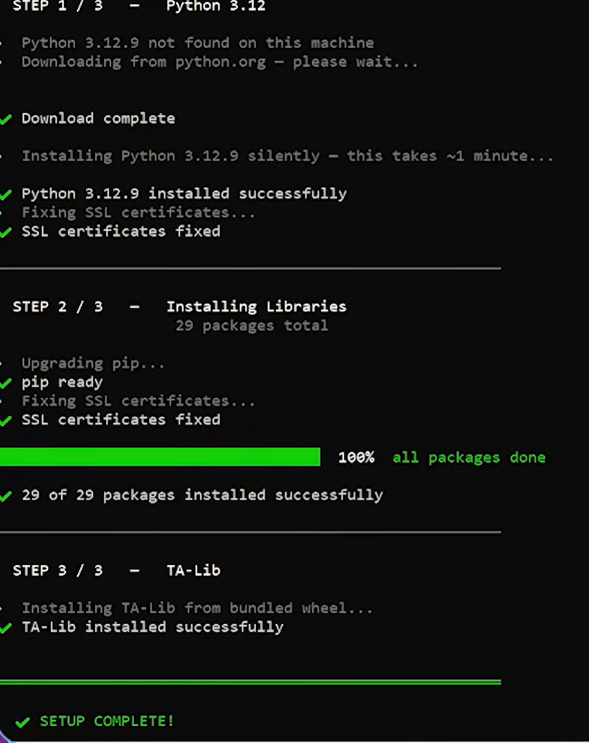
Figure 19: Step 1/3 downloads and silently installs Python 3.12.9; Step 2/3 installs all 29 required libraries; Step 3/3 installs TA-Lib from a bundled wheel — ending in “SETUP COMPLETE!”.

Once complete, the installer automatically opens Made For Trade, the community/support forum where all the code files for this series are posted and where questions can be asked directly.

Step 2 — Create a Made For Trade Account

Made For Trade is where trading- and algo-related questions can be asked, and where the code files for every part in this series are shared as replies in a dedicated thread.

Step 3 — Install Cursor

Cursor is an AI-based code editor used throughout the series for writing and running the algo code. It’s installed the same way — right-click → Run as Administrator — followed by a Google sign-in. A paid AI subscription (~$20/month) is recommended for at least the first month while still learning; it can be dropped once the underlying code is understood.

Inside Cursor: Ctrl+B opens the side panel, where the Python and “Sublime Text Keymap & Settings Importer” extensions should be installed.

Step 4 — Verify Python Is Working

Running test.py — a file that simply loops over the watchlist and prints a scan message for each symbol — confirms that Python is installed, Cursor recognizes it, and the environment is ready.

import datetime

watchlist = ["BEL", "TATACONSUM", "BAJAJ-AUTO", ...]  # full ~50-stock watchlist

for name in watchlist:
    current_time = datetime.datetime.now()
    print(f"I am dummy scanning for {name} at {current_time}")

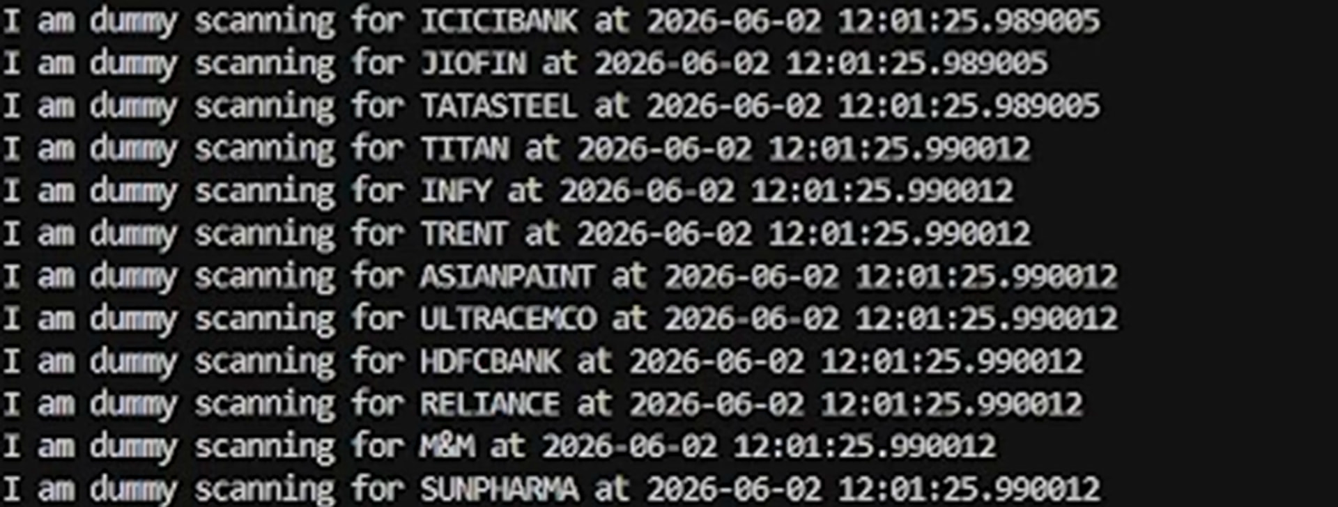
Figure 20: test.py output — a simple confirmation pass, scanning through the watchlist symbol by symbol.

Step 5 — Run demo_algo.py and Connect Your Dhan Account

The final file connects to Dhan and runs a basic RSI + EMA scanner. It needs three account-specific values filled in first:

Field	Where to get it
Client Code	Dhan → My Profile
PIN	Your Dhan login PIN
TOTP Secret	Dhan → Trading & Data APIs → Enable TOTP (scan the QR with an authenticator app)

tsl = Tradehull(ClientCode=client_code, mode="pin_totp", pin=pin, totp_secret=totp_secret)

for name in watchlist:
    try:
        chart = tsl.get_historical_data(
            tradingsymbol=name, exchange='NSE', timeframe="5"
        )
        chart['rsi'] = talib.RSI(chart['close'], timeperiod=14)
        chart['ema'] = talib.EMA(chart['close'], timeperiod=30)
        time.sleep(1)

        completed_candle = chart.iloc[-1]
        rsi   = completed_candle['rsi']
        ema   = completed_candle['ema']
        close = completed_candle['close']

        stock_in_bullish_momentum = (rsi > 60)
        stock_in_uptrend          = (close > ema)
        stock_in_bearish_momentum = (rsi < 40)
        stock_in_downtrend        = (close < ema)

        if stock_in_bullish_momentum and stock_in_uptrend:
            print(f"   I have a buy signal for {name} at {close}")

        if stock_in_bearish_momentum and stock_in_downtrend:
            print(f"   I have a sell signal for {name} at {close}")

    except Exception as e:
        continue

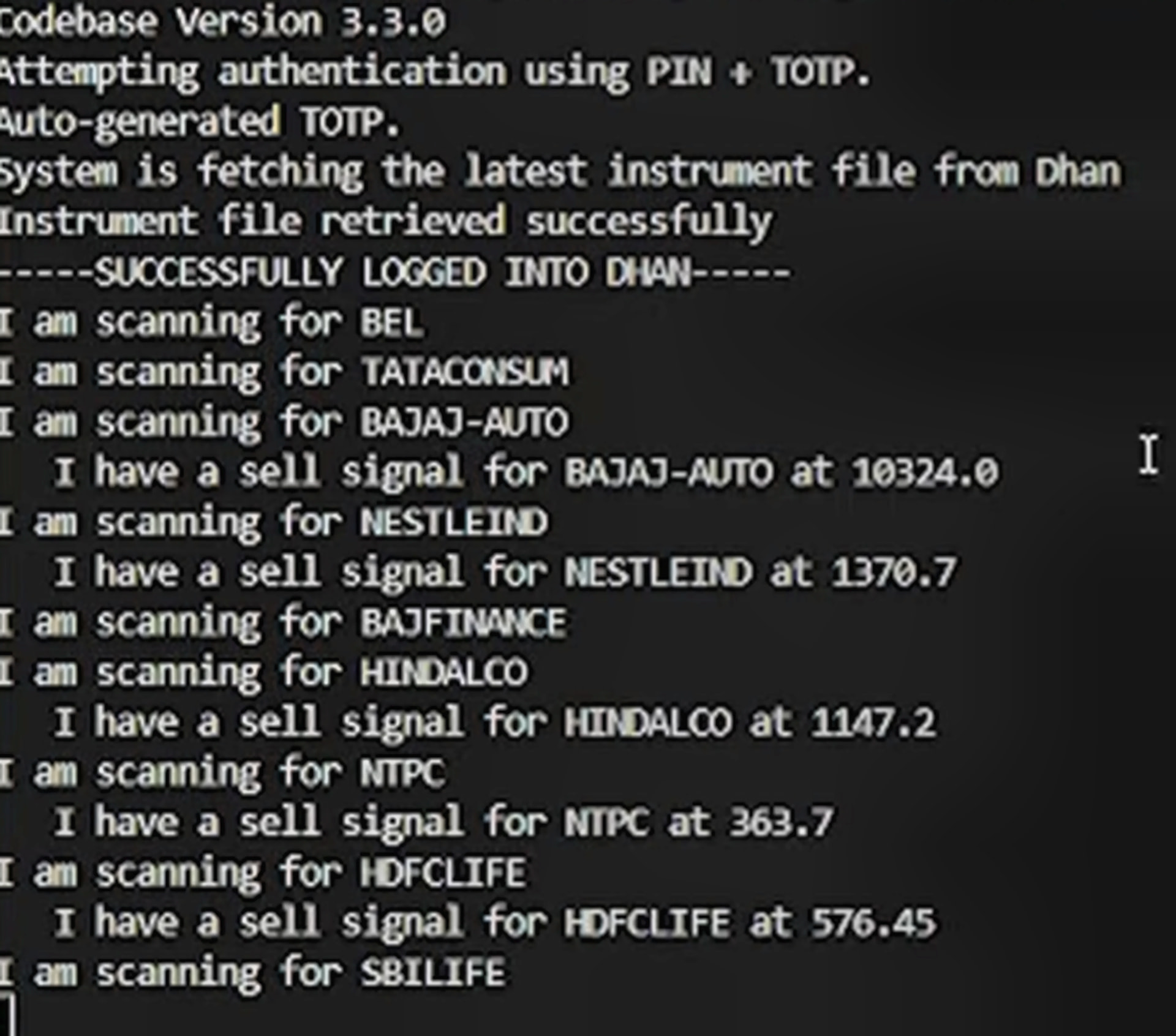
Figure 21: “SUCCESSFULLY LOGGED INTO DHAN” — the RSI + EMA scanner running live, flagging sell signals for Bajaj Auto, Nestle India, Hindalco, NTPC, and HDFC Life. No real orders are placed at this stage; the signals are print statements only, order placement comes in a later part.

If this step runs and produces output like the above, it confirms Python is installed, Cursor recognizes it, the Dhan API is connected, and live data is flowing into the account — the full local installation, end to end.

---

4. What’s Next

This part covered the API demo and installation only — no live orders are placed yet (order placement in this codebase also requires a static IP, covered in a later part of this series). The rest of the series builds on this foundation:

• Part 2: Python fundamentals for algo trading
• Part 3: Building a momentum scanner
• Part 4: Order placement + deploying the algo on Dhan Cloud
• Part 5: Extending the same algo to options and redeploying

---

Resources

• YouTube video: https://youtu.be/JEDAHxnFMak?si=mbJkrx4mKJF6oPJo
• Code files (Google Drive): https://drive.google.com/drive/folders/1TzsNsQO15HV4BFG4FBFxczNzumkt9r6O?usp=drive_link

---

Disclaimer: Investments in the securities market are subject to market risk. Read all related documents carefully before investing.